Systems of Linear Equations

We are interested in the solutions to systems of linear equations. A
linear equation is of the form

3x - 5y + 2z + w = 3.

The key thing is that we don't multiply the variables together nor do
we raise powers, nor takes logs or introduce sine and cosines. A system
of linear equations is of the form

3x - 5y + 2z = 3
-2x + y + 5z = -4.

This is a system of two linear equations in three variables. The first
equation is a system consisting of one linear equation in four variables.

In this class we will be more interested in the nature of the solutions
rather than the exact solutions themselves. So let us try to form a
picture of what to expect. Suppose we start with an easy case. A
system of two linear equations in two variables.

x - 2y = -1
2x + y = 3.

It is easy to check that this has the unique solution x = y = 1. To
see that this is not the only qualitative behaviour, suppose we consider
the system

2x + y = 3
2x + y = 3.

Since the second equation is precisely the same as the first equation,
it is enough to find x and y satisfying the system

2x + y = 3.

In other words the solution set is infinite. Any point of the line given
by the equation 2x + y = 3 will do. The problem is that the second
equation does not impose independent conditions. Note that we can
disguise (to a certain extent) this problem by writing down the system

2x + y = 3
4x + 2y = 6.

All we did was take the second equation and multiply it by 2. But we
are not fooled, we still realise that the second equation imposes no more
conditions than the first. It is not independent of the first equation.

We can tweak this example to get a system

2x + y = 3
2x + y = 2.

Now this system has no solutions whatsoever. If 2x + y = 3 then
2x + y ≠ 2. The key point is that these three examples exhaust the
qualitative behaviour.

• One solution.
• infinitely many solutions.
• No solutions.

In other words if there are at least two solutions then there are
infinitely many solutions. In particular it turns out that the answer
is never that there are two solutions. We say that a linear system is
inconsistent if there are no solutions and otherwise we also say that
the system is consistent.

It is instructive to think how this comes out geometrically. Suppose
there are two variables x and y. Then we can represent the solutions to
a system of linear equations in x and y as a set of points in the plane.
Points in the plane are represented by a pair of points (x, y) and we
will refer to these points as vectors. The set of all such points is called
R²,



Okay, so what are the possibilities for the solution set? Well suppose we
have a system of one equation. The solution set is a line. Suppose we
have a system of two equations. If the equations impose independent
conditions, then we get a single point, in fact the intersection of the two
lines represented by each equation. Are there other possible solution
sets? Yes, we already saw we might get no solutions. Either take a
system of two equations with no solutions (in fact parallel lines) or a
system of three equations, where we get three different points when we
intersect each pair of lines. If we have three equations can we still get
a solution? Yes suppose all three lines are concurrent (pass through
the same point). It is interesting to see how this works algebraically.
Suppose we consider the system

2x + y = 3
x - 2y = -1
3x - y = 2.

Then the vector (x, y) = (1, 1) still satisfies all three equations. Note
that the third equation is nothing more than the sum of the first two
equations. As soon as one realises this fact, it is clear that the third
equation fails to impose independent conditions, that is the third equa-
tion depends on the first two. Note one further possibility. The following
represents a system of three linear equations in two variables, with
a line of solutions.

x + y = 1
2x + 2y = 2
3x + 3y = 3.

These equations are very far from being independent. In fact no
matter how many equations there are, it is still possible (but more and
more unlikely) that there are solutions.

Finally let me point out some unusual possibilities. If we have a
system of no equations, then the solution set is the whole of R². In
fact

0x + 0y = 0,

represents a single equation whose solution set is R². By the same
token

0x + 0y = 1,

is a linear equation with no solutions.

In summary the solution set to a system of linear equations in two
variables exhibits one of four different qualitative possibilities.

(1) No solutions.
(2) One solution.
(3) A line of solutions.
(4) The whole plane R².

(Strictly speaking, so far we have only shown that these possibilities
occur, we have not shown that these are the only possibilities.). In
other words the case when there are infinitely many solutions can be
be further refined into the last two cases.

Now let us delve deeper into characterising the possible behaviour
of the solutions. Let us consider a system of three linear equations in
three unknowns. Can we list all geometric possibilities? One possibility
is we get a point. For example

The first equation cuts down the space of solutions to a plane, the
plane

The second equation represents another plane which intersects the first
plane in a line

The last equation defines a plane which intersects this line in the origin,
(0, 0, 0). Or the first two equations could give a line and the third
equation might also contain the same line,

The last equation is a sum of the first two equations. But we could
just as well consider

Again the problem is that the third equation is not independent from
the first two equations. There are many other possibilities. Two planes
could be parallel, in which case there are no solutions.

It is time for some general notation and definitions. A vector

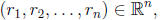
is a solution to a linear equation

if

A system of m linear equations in n variables has the form

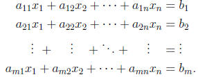
A solution to a system of linear equations is a vector
which satisfies all m equations simultaneously. The solution set
is the set of all solutions.

Okay let us now turn to the boring bit. Given a system of linear
equations, how does one solve the system? Again, let us start with a

simple example,

x - 2y = -1
2x + y = 3.

There are many ways to solve this system, but let me focus on a
particular method which generalises well to larger systems. Use the
first equation to eliminate x from the second equation. To do this,
take the first equation, multiply it by -2 and add it to the second
equation (we prefer to think of multiplying by a negative number and
adding rather than subtracting). We get a new system of equations,

x - 2y = -1
5y = 5.

Since the second equation does not involve x at all, it is straightforward
to use the second equation to get y = 1. Now use that value and
substitute it into the first equation to determine x,

x - 2 = -1,

so that x = 1. This method is called Gaussian elimination. The last
step, where we go from the bottom to the top and recursively solve for
the variables is called backwards substitution.

Let us do the same thing with a system of three equations in three
variables.

x - 2y - z = 4
2x - 3y + z = 10
-x + 5y + 11z = 3.

We start with the first equation and use it to eliminate the appearance
of x from the second equation. To do this, take the first equation,
multiply it by -2 and add it to the second equation.

x - 2y - z = 4
y + 3z = 2
-x + 5y + 11z = 3.