Algebra Potpourri
Don’t let the name of the program—The Geometer’s
Sketchpad—fool you.
Sketchpad has a host of tools for exploring algebra, trigonometry, and calculus,
both symbolically (with equations) and graphically. In this tour, you’ll sample
several of Sketchpad’s algebra features.
What You Will Learn
• How to create an x-y coordinate system and measure the coordinates of
a point
• How to define and plot functions
• How to plot two measurements as an (x, y) point in the plane
• How to construct a locus
A Simple Plot in the Coordinate (x-y) Plane
Presenter: Allow 10 minutes for the first two sections.
At the heart of “visual” algebra is the x-y (or Cartesian,
or coordinate) plane. In this
section, you’ll define a coordinate plane, measure a point’s coordinates on it,
and
plot a simple function.
1. Open a new sketch and choose Define Coordinate System
from the
Graph menu.
2. Using the Point tool, create a point somewhere other than on an axis.
3. With the point still selected, choose Coordinates from the Measure menu.
Drag the point to see how the coordinates change.
| Actually, you can plot
-> a function without first creating a coordinate system. Sketchpad creates coordinate systems automatically whenever needed. |
Now that there’s a
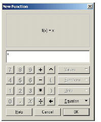
coordinate system, let’s plot a simple equation on it: y = x. 4. Choose Plot New Function from the Graph menu. 5. Click on x in the Function Calculator (or type x from your keyboard). Click OK. 6. Select the plot you just created and the independent point (whose coordinates you measured). Then choose Merge Point To Function Plot from the Edit menu. Drag the point along the plot and observe its coordinates. |
 |
| You may notice that -> the plot’s domain is restricted. To change the domain, drag the arrows at either end of the plot. |
7. Drag the unit point—the point at
(1, 0)—to the right and left and observe how the scale of the coordinate system changes. 8. Release the unit point when the x-axis goes from about –10 to 10. |
Plotting a Family of Curves with Parameters
Plotting one particular equation, y = x, is all well and
good. But the real power of
Sketchpad comes when you plot families of equations, such as the family of lines
of the form y = mx + b. You’ll start by defining parameters m and b and editing
the existing function equation to include the new parameters. Then you’ll
animate
the parameters to see a dynamic representation of this family of lines.
| A parameter is a -> type of variable that takes on a fixed value. |
9. Choose New Parameter
from the Graph menu. Enter m for Name and 2 for Value and click OK. 10. Use the same technique to create a parameter b with the value –1. |
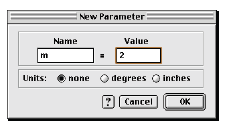 The New Parameter dialog box (Mac) |
| Edit Function -> appears as Edit Calculation, Edit Parameter, or Edit Plotted Point when one of those types of objects is selected. |
11. Select the function equation f (x) = x
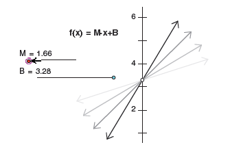
(select the equation itself, not its plot) and choose Edit Function from the Edit menu. 12. Edit the function to be f (x) = m ! x + b. (Click on the parameters m and b in the sketch to enter them. Use * from the Function Calculator or keyboard [Shift+8] for multiplication.) Click OK. 13. Change m and b (by double-clicking them) to explore several different graphs in the form y = mx + b, such as y = 5x + 2, y = –1x – 7, and y = 0.5x. |
You can learn a lot by changing the parameters manually,
as you did in the
previous step. But it can be especially revealing to watch the plot as its
parameters change smoothly or in steps.
14. Deselect all objects. Then select the parameter
equation for m and choose
Animate Parameter from the Display menu. What happens?
15. Press the Stop button to stop the
animation.
16. Select m and choose Properties from the
Edit menu. Go to the Parameter panel
and change the settings so they resemble
those at right. Click OK.
17. Again choose Animate Parameter.
18. Continue experimenting with parameter
animation. You might try, among other
things, animating both parameters
simultaneously or tracing the line as it
moves in the plane.
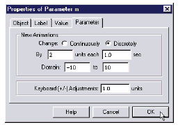
The Parameter Properties dialog box
(Windows)
Presenter: Stop here and answer questions. You may wish to
demonstrate modeling
y = mx + b using sliders instead of parameters (perhaps using sliders from the
sample
sketch Sliders.gsp). Allow about 15 minutes for the remainder of the activity.
Functions in a Circle
How does the radius of a circle relate to its
circumference? To its area? These are
examples of geometric relationships that can also be thought of as functions and
studied algebraically.
You’ll start by constructing a circle whose radius adjusts continuously along a
straight path.
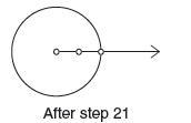
19. In a new sketch, use the Ray tool to construct a horizontal ray.
20. With the ray still selected, choose Point On Ray from the Construct menu.
21. With the Arrow tool, click in blank space to deselect all objects. Then
select,
in order, the ray’s endpoint and the point constructed in the previous step.
Choose Circle By Center+Point from the Construct menu.
| In each case, use -> the Arrow tool to select the circle (and nothing else), then choose the appropriate command in the Measure menu. |
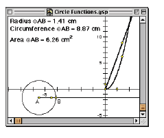
22. Measure the circle’s
radius, circumference, and area. 23. Drag the circle’s radius point and watch the measurements change. Next we’ll explore these measurements by plotting. 24. Select, in order, the radius measurement and the circumference measurement. Choose Plot As (x, y) from the Graph menu. Can you see your point? If not, it might be off the screen. |
 |
| In a rectangular -> grid, the x- and y-axes can be scaled independently. |
25. Choose Rectangular Grid from the Graph | Grid
Form submenu. Drag the new unit point at (0, 1) down until you can see the plotted point from the previous step. |
| Choose Erase -> Traces from the Display menu to erase this trace at any time |
26. Select the plotted point and choose Trace
Plotted Point from the Display menu. Drag the radius point and observe the trace. In situations such as this (where you trace something as a point moves along a path) you can often get a smoother picture by creating a locus. |
| A Sketchpad locus is -> a sample of possible locations of the selected object. To change the number of samples plotted, select the locus, choose Properties from the Edit menu, and go to the Plot panel. |
27. Select the plotted point and the
radius point; then choose Locus from the Construct menu. What is the slope of the line containing this locus? 28. Repeat steps 24 and 27, except this time explore the relationship between the radius and area measurements. How do the two curves compare? For what radius do the numerical values of a circle’s circumference and area equal each other (ignoring units)? |
 |
Further Challenges
• Graph pairs of parallel lines and show that their slopes are the same.
• Graph pairs of perpendicular lines and show that their slopes are negative
reciprocals.
• Graph a parabola of the form y = a(x – h)^2 + k, using parameters for a, h,
and k.